Research
Here are some brief outlines of some of my current and ongoing research projects and interests.
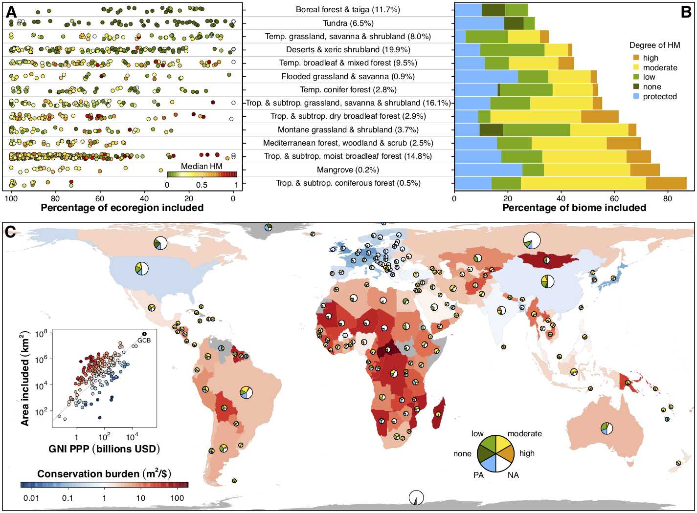
Spatial planning for global terrestrial and marine biodiversity conservation
The Half-Earth Project posits that we must set aside half of the earth for the successful preservation of biodiversity. I am using a spatial conservation planning framework to address the question most succinctly stated: “Which half?” Working closely with the E.O. Wilson Biodiversity Foundation and Map of Life, I combine global patterns of the distributions of 30,000+ terrestrial vertebrates with human land use layers, and use a linear optimization approach to design global conservation networks that protect a sufficient amount of habitat for every species. I am also doing a similar study for the marine environment, focusing on marine mammals and commonly harvested fish species.
Much of this research is designed to support the Convention on Biological Diversity and its associated Biodiversity Targets, and to help inform international negotiations of a post-2020 Global Biodiversity Framework, reflecting the best available science and most complete and up-to-date portrait of the planet’s biodiversity. A key feature of the results is that the burden of conservation is highly geographically variable, necessitating individualized conservation targets and goals at the national level as well as the species level.
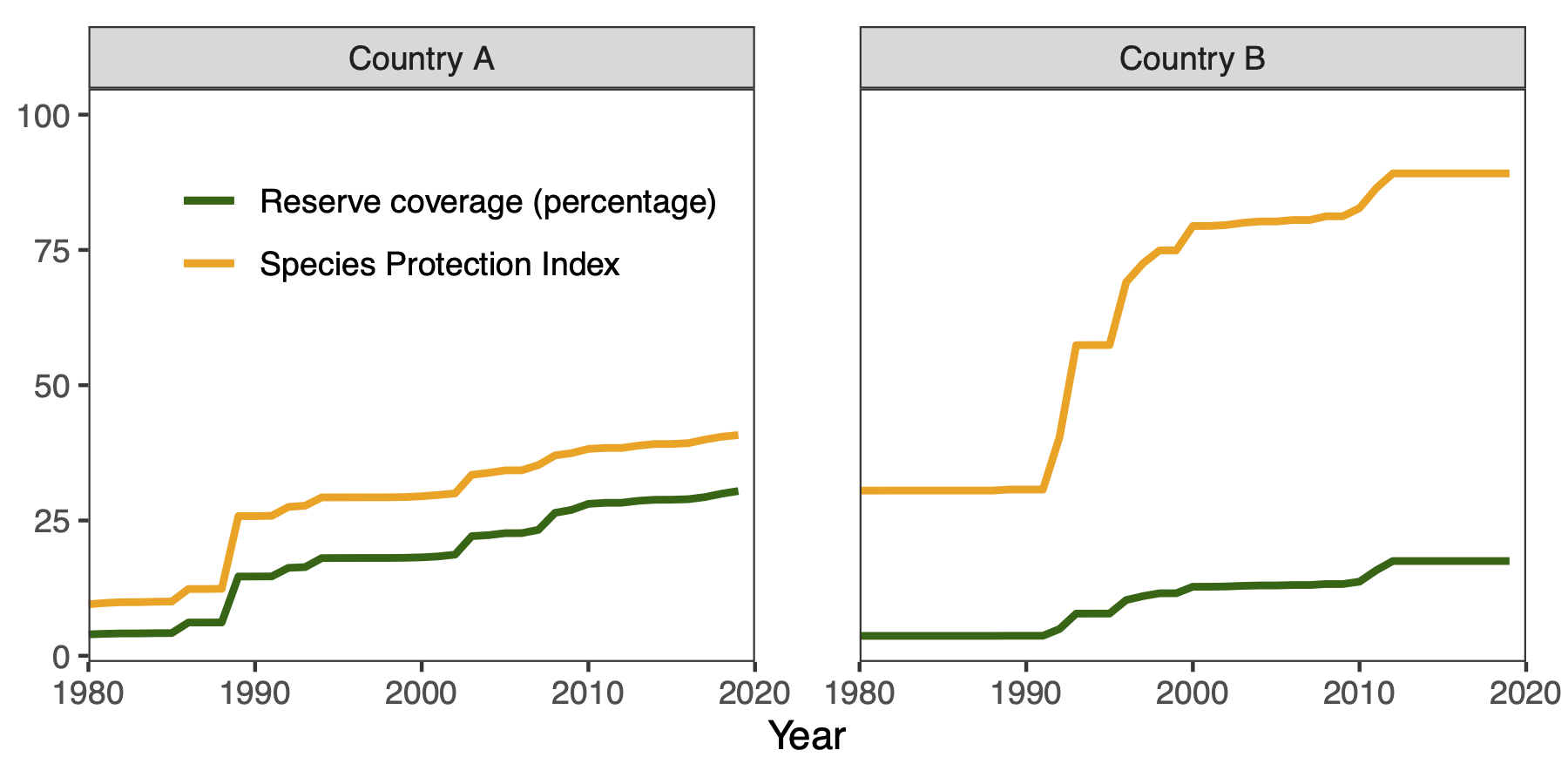
Biodiversity indicators for tracking conservation progress
Spatial conservation planning is a powerful tool for identifying how much protection is needed and where, but there is a distinction between identifying mathematically optimal solutions and turning solutions into action through real-world conservation policies and resource management. This process is slow and messy (in the best of times) due to additional considerations that may not have been accounted for in the modeling process, such as budgets, time horizons, conflicts with existing policies, and competing sociopolitical interests.
Biodiversity indicators are measurements derived from biodiversity data that enable us to study, report, and manage biodiversity change. I am part of a research team that creates these indicators for use in the conservation community, to better inform decision making helps ensure that our conservation actions continue to reflect and achieve our conservation goals through time by prioritizing areas where biodiversity protection is most needed. Our indicators have contributed to projects such as Yale’s Environmental Performance Index and the Half-Earth Project Map, and are currently under consideration for inclusion in the CBD’s post-2020 Global Biodiversity Framework as key indicators to track progress toward meeting Biodiversity Targets.
CENFA package for R: tools for climate- and environmental- niche factor analysis of spatial data
I authored and maintain an R package that provides methods for visualization of spatial variability of species sensitivity, exposure, and vulnerability to climate change. This package complements previous work of mine, and updates the ENFA method for use with large datasets and modern data formats. It also includes some functions for speeding up certain raster functions considerably via parallelization.
Available at https://cran.r-project.org/package=CENFA and https://github.com/rinnan/CENFA.
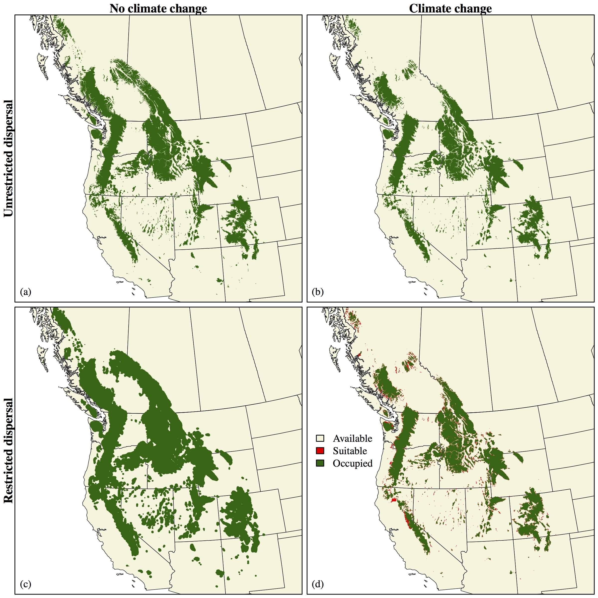
Incorporating biological and ecological realism into species distribution modeling
One common criticism of species distribution models (SDMs) is their lack of realism: describing the relationship between a species and its environment using only statistical correlations ignores all of the ecological and physiological processes that constrain the distributions of populations. By not accounting for dispersal ability, for example, SDMs fail to provide any insight into a species’ ability to successfully colonize new areas identified as potentially suitable future habitat. As such, SDMs can greatly underestimate species vulnerability to climate change.
Integro-difference equations (IDEs), by contrast, offer a modeling approach that provides a mechanistic understanding of how species traits shape long-term population dynamics. IDEs are quite flexible and can accommodate a wide variety of models, including stage-structure in populations, resource competition by multiple species, changes in habitat quality, density dependence, and environmental and demographic stochasticity. Despite their flexibility, integro-difference models are more theoretical in nature, and typically use an oversimplified notion of species habitat, often reducing it down to a single spatial dimension. While this is useful for understanding population dynamics and processes, it provides little insight into how these processes translate to a physical landscape.
I am developing and exploring a novel modeling framework that bridges the gap between these two approaches by combining the strengths of SDM and IDE techniques. This framework provides key insight into how traits such as growth rate and dispersal ability affect long-term population stability in a changing environment.